Results

Overall behavior

Using htpolynet plots we can generate a few interesting graphics that help characterize a build. In this tutorial, we generated a 95%-cure build under proj-0, with diagnostic output in diagnostics.log and console output to console.log.

As an exercise, copy pMSTY.yaml to pMSTY-low.yaml and in it, change the desired cure to 0.50 instead of 0.95. Then launch a second build:

$ htpolynet run -diag diagnostics-low.log pMSTY-low.yaml &> console-low.log

This will populate the project directory proj-1 (whose name is automatically assigned). Once it completes, we can generate some plots.

First, we can make plots of the conversion vs. run time and the cure iteration vs. run time:

$ htpolynet plots diag --diags diagnostics.log diagnostics-low.log

This generates cure_info.png:

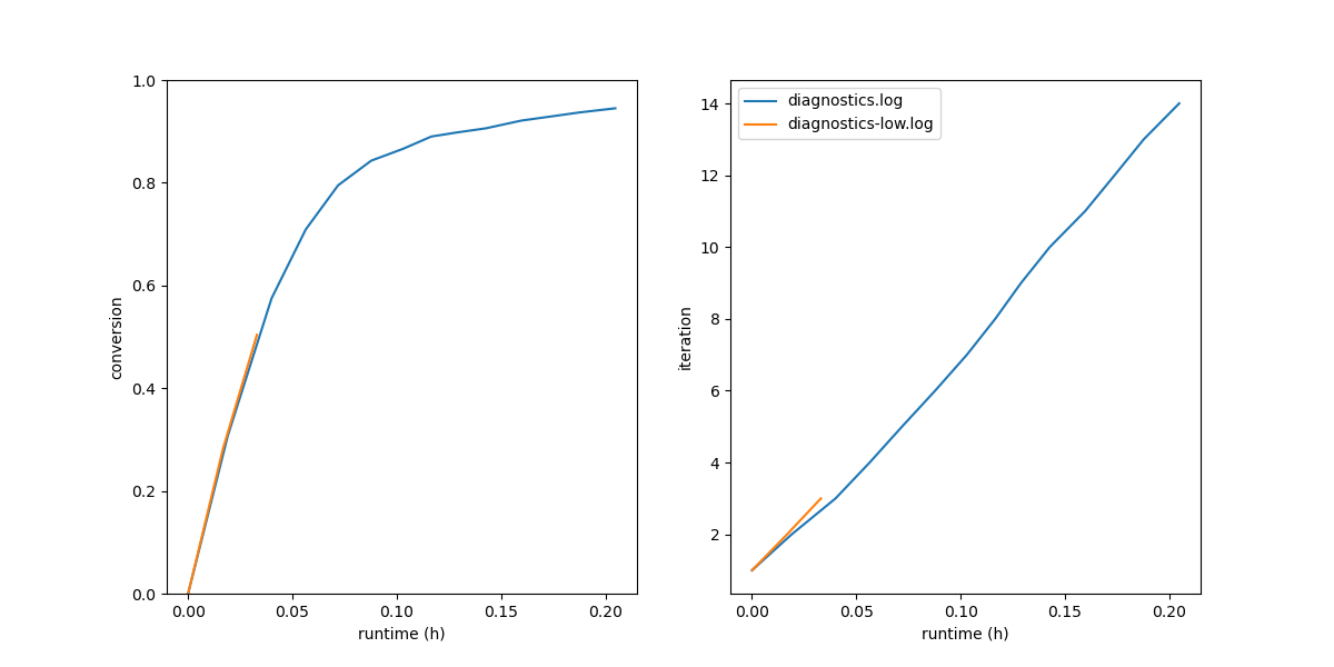
Fig. 7 (Left) Conversion vs. wall-clock time; (right) Iteration number vs wall-clock time.

We can see here that the 95% cure took about 8 and a half minutes of run time (which is not really impressive since this is a very small system). Fully two-thirds of the run time is consumed realizing the final 15% of the cure.

Second, we can make plots that track the temperature, density, and potential energy throughout the entire build process:

$ htpolynet plots build --proj proj-0 --buildplot t --traces t d p

This command extracts temperature, density, and potential energy from all Gromacs edr output files in proj-0/ in the order they were generated, plots them according to a default format, and stores the extracted data in a csv file. By default, the plot is in proj-0/buildtraces.png and the corresponding data in proj-0/buildtraces.csv.

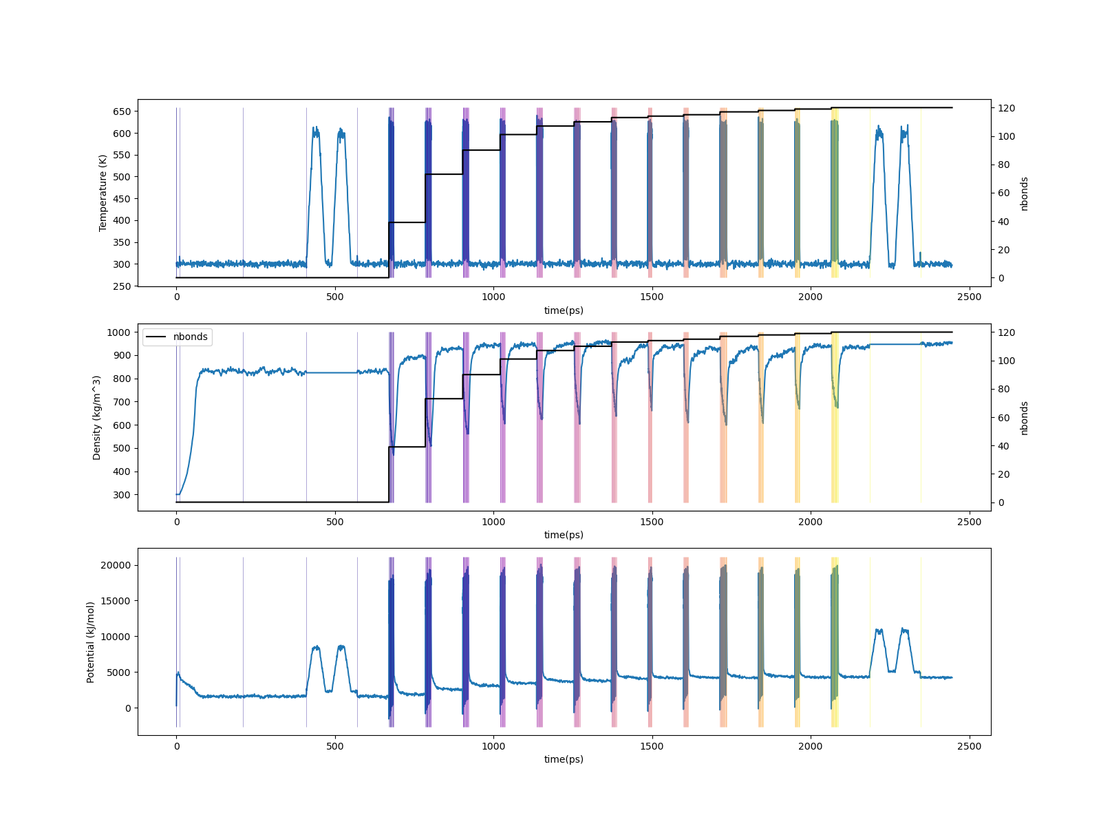
Fig. 8 (Top) Temperature vs. run time; (middle) Density vs. run time; (bottom) Potential energy vs. run time. In all panels, vertical lines designate initiations of Gromacs simulations.

From these traces, we can see how little MD time is actually devoted to forming the bonds as compared to relaxing both before and after. The top plot shows temperature in K vs. time in ps througout the build process. Vertical lines denote transitions from one step to the next; transitions are very close together in time during the CURE iterations since I’m showing one transition for each drag/relax stage. The middle plot shows the density trace’ note how the density begins at the stipulated low value of 300 kg/m3³. The bottom plot shows the potential energy trace.

In the figure below, we show two renderings of this system. In each, all bonds between C1 and C2 atoms are shown as grey tubes, and all other bonds are colored by individual unique monomer and made transparent. On the left is the system just after the precure anneal, where you can see that only intramolecular C1 and C2 bonds exist. On the right is the system after postcure, where you can see chains of -C1-C2- bonds.

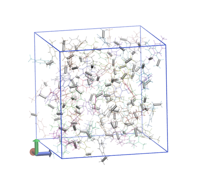
Fig. 9 Methystyrene liquid before cure.

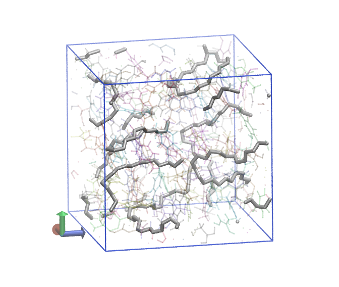
Fig. 10 Poly(methyl styrene) after 95% cure.

Details

The htpolynet run invocation in run.sh runs a high-cure build (95% conversion) in the proj-0 subdirectory, generating and populating the following directory structure:

$ cd proj-0
$ tree -d .
.
├── lib
│   └── molecules
│       ├── inputs
│       └── parameterized
└── proj-0
    ├── molecules
    │   └── parameterized
    ├── plots
    └── systems
        ├── capping
        ├── densification
        ├── final-results
        ├── init
        ├── iter-1
        ├── iter-10
        ├── iter-11
        ├── iter-12
        ├── iter-13
        ├── iter-2
        ├── iter-3
        ├── iter-4
        ├── iter-5
        ├── iter-6
        ├── iter-7
        ├── iter-8
        ├── iter-9
        ├── postcure
        └── precure

There are three main subdirectories in all project directories:

• molecules/: This directory has one subdirectory, molecules/parameterized that contains all files associated with generation and parameterization of all molecules and oligomer templates. The important files here are those with gro, top, itr, tpx, and grx extensions.

• systems/: This directory contains all directories where Gromacs runs are conducted.

• plots/: This directory contains some plots generated on the fly.

proj-0/systems

The init/ directory is where the initial topology and coordinates are generated.

$ ls systems/init
EMB.gro  init.gro  init.grx  init.top

Then in densification are the files associated with the MD simulations used to densify the initial system.

$ ls systems/densification
densified-min.edr  densified-npt.edr  densified-nvt.edr  init.grx
densified-min.gro  densified-npt.gro  densified-nvt.gro  init.top
densified-min.log  densified-npt.log  densified-nvt.log  init.tpx
densified-min.mdp  densified-npt.mdp  densified-nvt.mdp  mdout.mdp
densified-min.tpr  densified-npt.tpr  densified-nvt.tpr  min.mdp
densified-min.trr  densified-npt.trr  densified-nvt.trr  npt.mdp
densified-npt.cpt  densified-nvt.cpt  init.gro           nvt.mdp

The files with init basenames are copied from the systems/init directory. You can note output from three separate Gromacs mdrun invocations: 1. a minimization; 2. an NVT equilibration, and 3. an NPT equilibration.

Next comes the precure directory, which contains all the results of the precure equilibrations and annealing (if requested).

$ ls systems/precure
annealed.cpt               postequilibration-npt.edr
annealed.edr               postequilibration-npt.gro
annealed.gro               postequilibration-npt.log
annealed.log               postequilibration-npt.mdp
annealed.tpr               postequilibration-npt.tpr
annealed.trr               postequilibration-npt.trr
densified-npt.gro          preequilibration-npt.cpt
init.grx                   preequilibration-npt.edr
init.top                   preequilibration-npt.gro
init.tpx                   preequilibration-npt.log
mdout.mdp                  preequilibration-npt.mdp
npt.mdp                    preequilibration-npt.tpr
nvt.mdp                    preequilibration-npt.trr
postequilibration-npt.cpt

Here, init.top, init.tpx, and init.grx are copied from systems/densification, as is coordinate file densified-npt.gro. These are input to the pre-annealing equilibration (preequilibration-npt.*), which then serves as input to the annealing simulation (annealed.*), which in turn serves as input to the post-annealing equilibration (postequilibration-npt.*).

Next come the iteration directories; here, thirteen CURE iterations were run. Below we show just a listing of the iter-1 directory.

$ ls systems/iter-1
0-cure_bondsearch-bonds.csv   3-cure_relax-stage-1-nvt.tpr  3-cure_relax-stage-3-min.tpr  3-cure_relax-stage-4-npt.tpr  3-cure_relax-stage-5-nvt.tpr
2-cure_update-bonds.csv       3-cure_relax-stage-1-nvt.trr  3-cure_relax-stage-3-min.trr  3-cure_relax-stage-4-npt.trr  3-cure_relax-stage-5-nvt.trr
2-cure_update.gro             3-cure_relax-stage-1.top      3-cure_relax-stage-3-npt.cpt  3-cure_relax-stage-4-nvt.cpt  3-cure_relax-stage-5.top
2-cure_update.grx             3-cure_relax-stage-2-min.edr  3-cure_relax-stage-3-npt.edr  3-cure_relax-stage-4-nvt.edr  4-cure_equilibrate-npt.cpt
2-cure_update-idx-mapper.csv  3-cure_relax-stage-2-min.gro  3-cure_relax-stage-3-npt.gro  3-cure_relax-stage-4-nvt.gro  4-cure_equilibrate-npt.edr
2-cure_update.top             3-cure_relax-stage-2-min.log  3-cure_relax-stage-3-npt.log  3-cure_relax-stage-4-nvt.log  4-cure_equilibrate-npt.gro
2-cure_update.tpx             3-cure_relax-stage-2-min.tpr  3-cure_relax-stage-3-npt.tpr  3-cure_relax-stage-4-nvt.tpr  4-cure_equilibrate-npt.log
3-cure_relax-complete.top     3-cure_relax-stage-2-min.trr  3-cure_relax-stage-3-npt.trr  3-cure_relax-stage-4-nvt.trr  4-cure_equilibrate-npt.mdp
3-cure_relax-relax-bonds.csv  3-cure_relax-stage-2-npt.cpt  3-cure_relax-stage-3-nvt.cpt  3-cure_relax-stage-4.top      4-cure_equilibrate-npt.tpr
3-cure_relax-stage-1-min.edr  3-cure_relax-stage-2-npt.edr  3-cure_relax-stage-3-nvt.edr  3-cure_relax-stage-5-min.edr  4-cure_equilibrate-npt.trr
3-cure_relax-stage-1-min.gro  3-cure_relax-stage-2-npt.gro  3-cure_relax-stage-3-nvt.gro  3-cure_relax-stage-5-min.gro  init.grx
3-cure_relax-stage-1-min.log  3-cure_relax-stage-2-npt.log  3-cure_relax-stage-3-nvt.log  3-cure_relax-stage-5-min.log  init.top
3-cure_relax-stage-1-min.tpr  3-cure_relax-stage-2-npt.tpr  3-cure_relax-stage-3-nvt.tpr  3-cure_relax-stage-5-min.tpr  init.tpx
3-cure_relax-stage-1-min.trr  3-cure_relax-stage-2-npt.trr  3-cure_relax-stage-3-nvt.trr  3-cure_relax-stage-5-min.trr  linkcell-0.50.grx
3-cure_relax-stage-1-npt.cpt  3-cure_relax-stage-2-nvt.cpt  3-cure_relax-stage-3.top      3-cure_relax-stage-5-npt.cpt  mdout.mdp
3-cure_relax-stage-1-npt.edr  3-cure_relax-stage-2-nvt.edr  3-cure_relax-stage-4-min.edr  3-cure_relax-stage-5-npt.edr  npt.mdp
3-cure_relax-stage-1-npt.gro  3-cure_relax-stage-2-nvt.gro  3-cure_relax-stage-4-min.gro  3-cure_relax-stage-5-npt.gro  postequilibration-npt.gro
3-cure_relax-stage-1-npt.log  3-cure_relax-stage-2-nvt.log  3-cure_relax-stage-4-min.log  3-cure_relax-stage-5-npt.log  relax-min.mdp
3-cure_relax-stage-1-npt.tpr  3-cure_relax-stage-2-nvt.tpr  3-cure_relax-stage-4-min.tpr  3-cure_relax-stage-5-npt.tpr  relax-npt.mdp
3-cure_relax-stage-1-npt.trr  3-cure_relax-stage-2-nvt.trr  3-cure_relax-stage-4-min.trr  3-cure_relax-stage-5-npt.trr  relax-nvt.mdp
3-cure_relax-stage-1-nvt.cpt  3-cure_relax-stage-2.top      3-cure_relax-stage-4-npt.cpt  3-cure_relax-stage-5-nvt.cpt
3-cure_relax-stage-1-nvt.edr  3-cure_relax-stage-3-min.edr  3-cure_relax-stage-4-npt.edr  3-cure_relax-stage-5-nvt.edr
3-cure_relax-stage-1-nvt.gro  3-cure_relax-stage-3-min.gro  3-cure_relax-stage-4-npt.gro  3-cure_relax-stage-5-nvt.gro
3-cure_relax-stage-1-nvt.log  3-cure_relax-stage-3-min.log  3-cure_relax-stage-4-npt.log  3-cure_relax-stage-5-nvt.log

Files in iteration directories are prepended with a number that corresponds to their order. Here we have files that begin with 0, 2, and 3. “0” refers to the initial search for possible bonds; these are reported in the csv file. “1” (which is missing here) refers to pre-bond dragging; since no new bonds were longer than 0.8 nm, pre-bond dragging was not triggered. “2” refers to the generation of the new bonded topology. “3” refers to post-bond-formation relaxation to allow new bonds to relax to their equilibrium lengths. These relaxations progress through five iterations of minimization-NVT-NPT simulations to relax the new bonds.

Some CURE iterations may require pre-bond dragging. In the system I ran to generate this documentation, no cases of prebond dragging were required.

Then comes the capping directory where the final topology updates are performed to cap any unreacted monomers (reverting them from their “active” forms to their “proper” forms). In this run, this directory is empty, since no unreacted monomers exist at the end of the CURE.

Then comes postcure equilibration and relaxation.

$ ls systems/postcure
2-cure_update.grx           mdout.mdp
2-cure_update.tpx           npt.mdp
3-cure_relax-complete.top   nvt.mdp
4-cure_equilibrate-npt.gro  postequilibration-npt.cpt
annealed.cpt                postequilibration-npt.edr
annealed.edr                postequilibration-npt.gro
annealed.gro                postequilibration-npt.log
annealed.log                postequilibration-npt.mdp
annealed.tpr                postequilibration-npt.tpr
annealed.trr                postequilibration-npt.trr

The files beginning with digits are copied either from the last iter directory or the capping directory (here, since no capping was necessary, they came from iter-13). As stipulated in the configuration file, we first run annealing, and then a post-annealing NPT equilibration.

Finally, HTPolyNet copies the results of the postcure, with new file names, into final-results.

$ ls final-results
final.gro  final.grx  final.top  final.tpx

Here we see the top, gro, tpx, and grx files of the final system; the top and gro files can be used right away for Gromacs MD simulations.

proj-0/plots

HTPolyNet generates several plots on the fly during a system build.

$ ls plots
densification-density.png
iter-10-cure_equilibrate-density.png
iter-11-cure_equilibrate-density.png
iter-12-cure_equilibrate-density.png
iter-13-cure_equilibrate-density.png
iter-1-cure_equilibrate-density.png
iter-2-cure_equilibrate-density.png
iter-3-cure_equilibrate-density.png
iter-4-cure_equilibrate-density.png
iter-5-cure_equilibrate-density.png
iter-6-cure_equilibrate-density.png
iter-7-cure_equilibrate-density.png
iter-8-cure_equilibrate-density.png
iter-9-cure_equilibrate-density.png
postcure-anneal-T.png
postcure-postequilibration-density.png
precure-anneal-T.png
precure-postequilibration-density.png
precure-preequilibration-density.png
reaction_network.png

For example, densification-density.png indicates that the densification simulation was in fact able to densify the system:

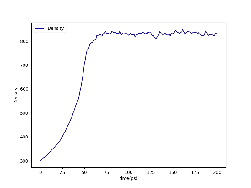
Fig. 11 densification-density.png for the high-cure build of polymethylstyrene.

We can check that the annealing cycles were correctly performed from precure-anneal-T.png postcure-anneal-T.png:

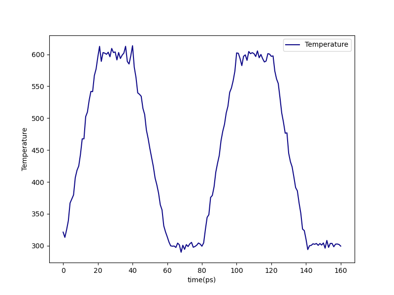
Fig. 12 Temperature during pre-cure annealing.

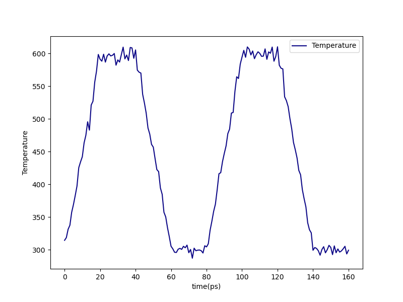
Fig. 13 Temperature during post-cure annealing.

Finally, we can take a look at the density after the postcure-anneal in postcure-postequilibration-density.png:

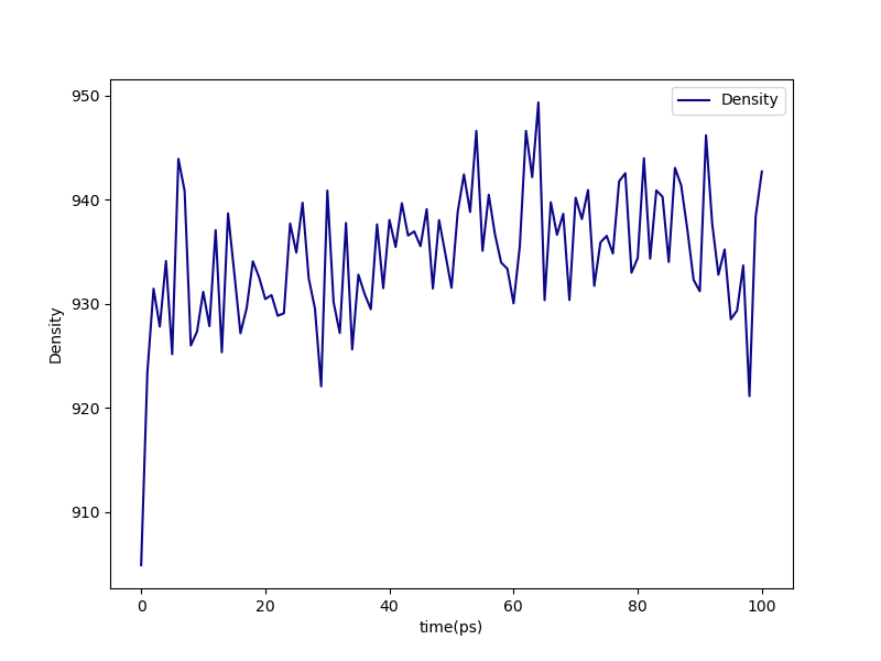
Fig. 14 postcure-postequilibration-density.png

Density during post-cure annealing of the 95% cured system.

Note that the final equilibrated density at 300 K and 1 bar is about 935 kg/m³. This is quite a bit higher than the density of liquid styrene at 10 bar and 300 K from the densification simulations (about 800 kg/m³). However, this result is outside the range expected for poly(4-methyl styrene) of about 1.01 g/cc, but it’s not too suprising given that this is a very small system with a low molecular weight, and it was not very extensively equilibrated.